Using D3 Quadtrees to Power An Interactive Map for Bonnier Corporation

Here at Phase2 we are working with D3.js more and more  as a tool for creating beautiful data visualizations. Overall, we're happy with the variety of ways we can use these building blocks to create very interesting and informative graphics.

Like all good engineers, we're eager to find new uses for our favorite toolsets.

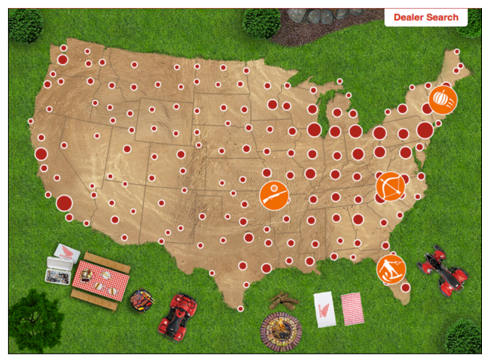
Recently I was able to work on a team with the folks at Bonnier Corporation to create a map for a custom marketing campaign. Working on a team with Danny and Joey Groh, we designed and implemented an interactive map in no time flat.

Why make maps in D3?

D3 comes with a variety of tools to make really interesting SVG-based maps. Unlike working with SVG directly, it's fairly straightforward to take geocoded information (via GeoJSON) and convert that into path components that D3 can handle. Unlike more traditional online mapping tools like Google Maps or Mapbox, D3 is simple to integrate with other visualizations. It's also able to handle many different map projections to better suit visualizations where the typical Mercator-type projection isn't appropriate.

Other libraries like Openlayers or Leaflet have some great plugins to do point clustering for us. Unfortunately in D3, there is no straightforward way to do point clustering. This proved to be one of our main challenges.

What is point clustering? What's a quad-tree?

Point clustering is the process of paring down a large number of points on a plane to a smaller set. There are a few reasons why you might want to do this. Visually, it's very difficult to actually get any real sense of what's happening on a map if it's just a sea of points. Additionally, from a performance perspective, rendering thousands of points on a map can be a real drag for your browser, since it has to actually process each point in the DOM.

Point clustering is the basic process of finding the nearest neighbors of each point and grouping them together. The easiest way to visualize this is to picture a grid over your map.

Each grid element should have a set number of points in it. A clustered point would be the average position of each point inside of each of the grid elements.

When we're dealing with a large amount of data, we need to find ways to process it more quickly. One way to do that is to filter down the number of points you need to search in order to check each grid item on the page.

One great way to do that is to use a data structure called a quadtree to store your point information. Quadtrees are helpful because they organize your data in such a way so that you can search for a whole set of data, rather than each individual point. By doing this, you can dramatically reduce the amount of time you spend searching.

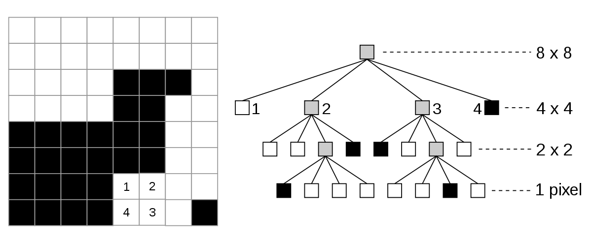
"Quad tree bitmap" by Wojciech Muła - Own work. Licensed under Public domain via Wikimedia Commons.

Step By Step

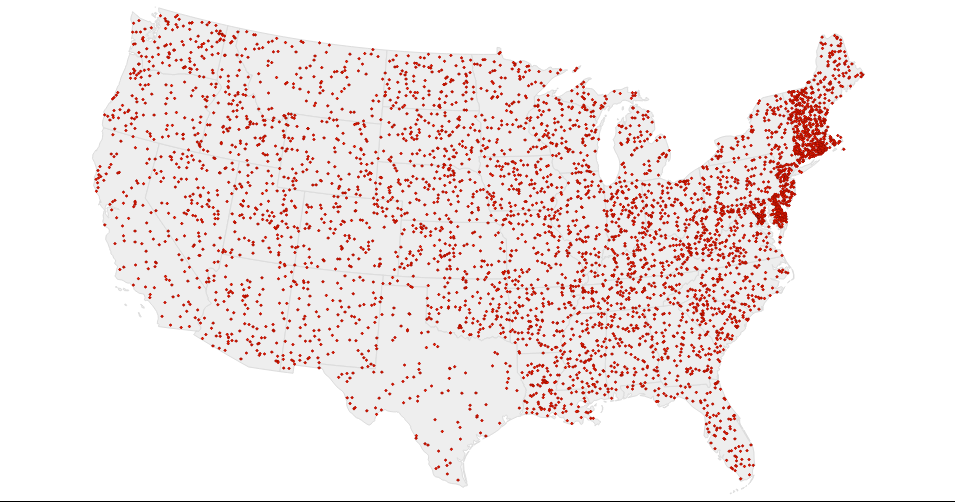
Now I’d like to demonstrate how to reduce a large dataset to a more manageable number of points for a map. I created our dataset by plotting 5,000 random points across the United States. 5,000 is a good number, because it's too many data points to really make visual sense on a map, but still well within the range of being manageable in D3.

Step 1. Setting up the map

There are plenty of great tutorials out there in the world about setting up maps with D3, so we'll skip the basics. Here's the basic javascript I've used to initially set up the map.

var width = 960,
 height = 500;

var svg = d3.select("#map").append("svg")
 .attr("width", width)
 .attr("height", height);

var g = svg.append("g");

var projection = d3.geo.albers();
var path = d3.geo.path().projection(projection).pointRadius(1);

d3.json("json/data.json", function(error, geoData) {
 if (error) return console.error(error);

 var points = topojson.feature(geoData, geoData.objects.points);
 var states = topojson.feature(geoData, geoData.objects.states);

 g.selectAll(".state")
   .data(states.features)
   .enter().append("path")
   .attr("class", function(d) {return "state state-" + d.properties.postal;})
   .attr("d", path);

 g.selectAll(".point")
   .data(points.features)
   .enter().append("path")
   .attr("class", "point")
   .attr("d", path);
});

As you can see with our initial map, it's pretty difficult to actually tell what's going on with the map beyond "Wow, there's a lot of data here." Again, this is a random data set, so there's not much going on here anyway, but if this were a real dataset, it would still be hard to understand.

Step 2: Defining our Grid

So, to get us going, we need to first define what our grid looks like. One thing to note is that our grid is set based on the SVG coordinates and not by geospatial coordinates, which means we're looking at dividing the screen up by what we can actually see on the screen, versus a translation to the underlying latitude/longitude points for the underlying data.

For our map, I've chosen to create a 45 by 45 grid. 

Here's what that looks like from a code perspective.

 var clusterPoints = [];
 var clusterRange = 45;

 var grid = svg.append('g')
   .attr('class', 'grid');

 for (var x = 0; x <= width; x += clusterRange) {
   for (var y = 0; y <= height; y+= clusterRange) {
     grid.append('rect')
       .attr({
         x: x,
         y: y,
         width: clusterRange,
         height: clusterRange,
         class: "grid"
       });
   }
 }

Step 3: Add our data to a quadtree and cluster

Now that we have a grid defined, let's start clustering our data. Like I mentioned before, we want to add our data to a quadtree in order to make it faster to search. D3 has a great implementation built in, and adding our data to the quadtree is pretty straightforward.

var pointsRaw = points.features.map(function(d, i) {
  var point = path.centroid(d);
  point.push(i);
  return point;
});
quadtree = d3.geom.quadtree()(pointsRaw);

The first bit of code creates an array of arrays that contains the x and y coordinates based on the geospatial coordinates. In addition, I'm adding the index of the individual feature to the data structure so that we can reference the original data if we need to later on. The last line of code creates the actual quadtree.

From there, we need to actually generate the clustered points and drop them on the map. To do this, we're going to borrow liberally from this great example of how to use quadtrees in D3.

// Find the nodes within the specified rectangle.
 function search(quadtree, x0, y0, x3, y3) {
   var validData = [];
   quadtree.visit(function(node, x1, y1, x2, y2) {
     var p = node.point;
     if (p) {
       p.selected = (p[0] >= x0) && (p[0] < x3) && (p[1] >= y0) && (p[1] < y3);
       if (p.selected) {
         validData.push(p);
       }
     }
     return x1 >= x3 || y1 >= y3 || x2 < x0 || y2 < y0;
   });
   return validData;
 }

 var clusterPoints = [];
 var clusterRange = 45;

 for (var x = 0; x <= width; x += clusterRange) {
   for (var y = 0; y <= height; y+= clusterRange) {
     var searched = search(quadtree, x, y, x + clusterRange, y + clusterRange);

     var centerPoint = searched.reduce(function(prev, current) {
       return [prev[0] + current[0], prev[1] + current[1]];
     }, [0, 0]);

     centerPoint[0] = centerPoint[0] / searched.length;
     centerPoint[1] = centerPoint[1] / searched.length;
     centerPoint.push(searched);

     if (centerPoint[0] && centerPoint[1]) {
       clusterPoints.push(centerPoint);
     }
   }
 }

 g.selectAll(".centerPoint")
   .data(clusterPoints)
   .enter().append("circle")
   .attr("class", function(d) {return "centerPoint"})
   .attr("cx", function(d) {return d[0];})
   .attr("cy", function(d) {return d[1];})
   .attr("fill", '#FFA500')
   .attr("r", 6)
   .on("click", function(d, i) {
     console.log(d);
   })

The first function 'search' will transverse the quadtree and will return an array of all the data points that are found in an individual grid item. The next set of for loops that start on line 20 loop through each grid element on the graphic. Lines 24-30 finds the average location of all the points that have been found in that particular grid item and adds the actual point to an extra element in the array for later lookup. Lines 32-34 adds a point to a running list if we have a valid point. In this particular implementation, this happens when there are no points in a particular grid item.

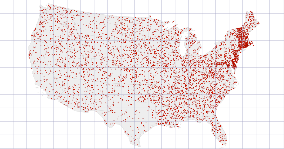
Here's what this looks like so far, along with a visualization of the underlying quadtree.

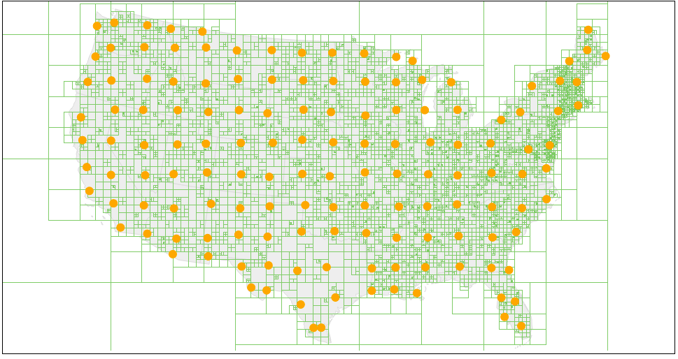
Step 4: Adjust the size

At this point, we're pretty close, but we can do better. Each point is being rendered the same way, and there's nothing that shows the amount of data each cluster point represents. There's a few different ways we could visually encode this, but in this case we’ll simply adjust the size of each point.

First, create a linear scale based on the data.

var pointSizeScale = d3.scale.linear()
   .domain([
     d3.min(clusterPoints, function(d) {return d[2].length;}),
     d3.max(clusterPoints, function(d) {return d[2].length;})
   ])
   .rangeRound([3, 15]);

After that, adjusting the size is pretty straightforward.

g.selectAll(".centerPoint")
   .data(clusterPoints)
   .enter().append("circle")
   .attr("class", function(d) {return "centerPoint"})
   .attr("cx", function(d) {return d[0];})
   .attr("cy", function(d) {return d[1];})
   .attr("fill", '#FFA500')
   .attr("r", function(d, i) {return pointSizeScale(d[2].length);})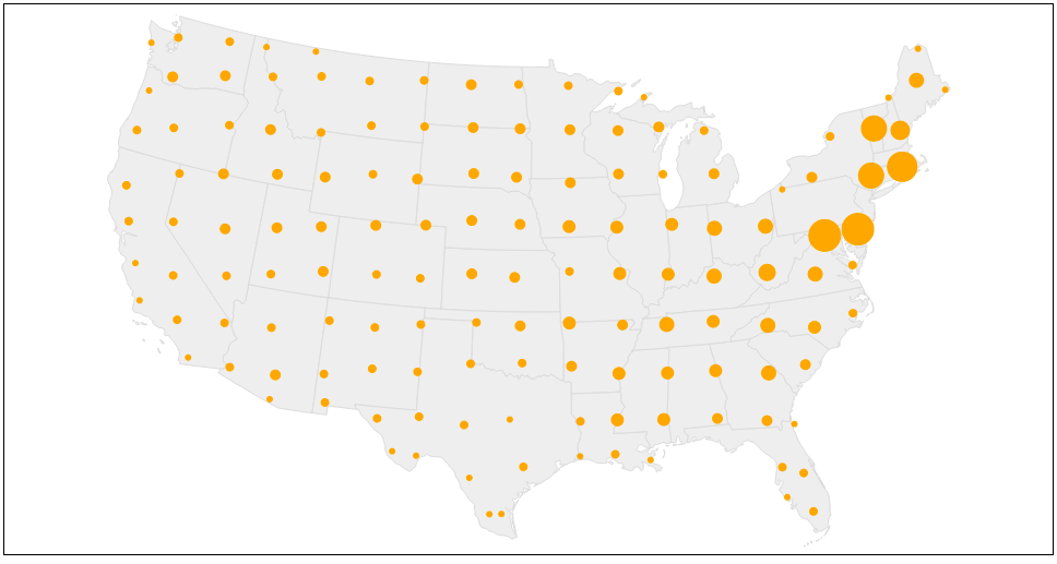

Next Steps

There are plenty of directions to go from here. You could show a listing of the exact number of elements in each cluster point via an overlaid number. Since you have access to the original data, you could show an overlay with an alternative view or list the original data set. If you wanted to get really crazy, you could use D3 transitions to add a toggle to adjust the size of your grid to dynamically animate the points.

If you want to check out an example of how this works, check out the companion repo on github.

Resources

• http://jimkang.com/quadtreevis/ - A great intro to quadtrees in general.
• http://bl.ocks.org/emeeks/7d5925cb7d9721c60360 - An alternate D3 clustering implementation tied to d3.carto.map
• http://bl.ocks.org/mbostock/4343214 - Great example of how to duse the core quadtree functionality in D3.
• http://robots.thoughtbot.com/how-to-handle-large-amounts-of-data-on-maps - A great blog post by the gang at Thoughtbot on doing map clustering in their iOS application.